片持梁の検証
![]()
有限要素法ライブラリGetFEM ++.を使用した片持ち梁について考えます。
モデルの作成
これで準備ができました。ライブラリをインポートします。
[1]:
import getfem as gf
import numpy as np
import numpy.testing as npt
import pandas as pd
import pyvista as pv
from IPython.display import Markdown

from pyvirtualdisplay import Display
import os
display = Display(visible=0, size=(1280, 1024))
display.start()
[1]:
<pyvirtualdisplay.display.Display at 0x7ff96dbb9d90>
The review cases are as follows. GetFEM++ uses FEM_PRODUCT and IM_PRODUCT to two-dimensional the finite element method and the integration method, respectively. For quadratic elements, the Gaussian integration point is 3. IM_GAUSS1D(K) represents the integration point of \(K/2+1\) points. The element uses plane strain elements. Set up these meshes, the finite element method and the integration method.
[2]:
cases = [
    "case11",
    "case12",
    "case13",
    "case14",
    "case21",
    "case22",
    "case23",
    "case24",
    "case31",
    "case32",
    "case33",
    "case34",
    "case41",
    "case42",
    "case43",
    "case44",
]
[3]:
xs = [
    4,
    4,
    4,
    16,
    4,
    4,
    4,
    16,
    4,
    4,
    4,
    16,
    4,
    4,
    4,
    16,
]
ys = [
    1,
    2,
    4,
    8,
    1,
    2,
    4,
    8,
    1,
    2,
    4,
    8,
    1,
    2,
    4,
    8,
]
[4]:
fem_names = [
    "FEM_PK(1, 2)",
    "FEM_PK(1, 2)",
    "FEM_PK(1, 2)",
    "FEM_PK(1, 2)",
    "FEM_PK(1, 1)",
    "FEM_PK(1, 1)",
    "FEM_PK(1, 1)",
    "FEM_PK(1, 1)",
    "FEM_PK(1, 1)",
    "FEM_PK(1, 1)",
    "FEM_PK(1, 1)",
    "FEM_PK(1, 1)",
    "FEM_PK_WITH_CUBIC_BUBBLE(1, 1)",
    "FEM_PK_WITH_CUBIC_BUBBLE(1, 1)",
    "FEM_PK_WITH_CUBIC_BUBBLE(1, 1)",
    "FEM_PK_WITH_CUBIC_BUBBLE(1, 1)",
]
[5]:
methods = [
    "IM_GAUSS1D(4)",
    "IM_GAUSS1D(4)",
    "IM_GAUSS1D(4)",
    "IM_GAUSS1D(4)",
    "IM_GAUSS1D(2)",
    "IM_GAUSS1D(2)",
    "IM_GAUSS1D(2)",
    "IM_GAUSS1D(2)",
    "IM_GAUSS1D(0)",
    "IM_GAUSS1D(0)",
    "IM_GAUSS1D(0)",
    "IM_GAUSS1D(0)",
    "IM_GAUSS1D(4)",
    "IM_GAUSS1D(4)",
    "IM_GAUSS1D(4)",
    "IM_GAUSS1D(4)",
]
[6]:
pd.options.display.float_format = "{:.2f}".format
data = []
columns = ["Case Name", "Mesh", "Finite Element Method", "Integration Method"]
for case, x, y, fem_name, method in zip(cases, xs, ys, fem_names, methods):
    data.append([case, str(x) + "x" + str(y), fem_name, method])
df = pd.DataFrame(data=data, columns=columns)
Markdown(df.to_markdown())
[6]:
| ケース名 | メッシュ | 有限要素法 | 積分法 | |
|---|---|---|---|---|
| 0 | case11 | 4x1 | FEM_PK(1, 2) | IM_GAUSS1D(4) |
| 1 | case12 | 4x2 | FEM_PK(1, 2) | IM_GAUSS1D(4) |
| 2 | case13 | 4x4 | FEM_PK(1, 2) | IM_GAUSS1D(4) |
| 3 | case14 | 16x8 | FEM_PK(1, 2) | IM_GAUSS1D(4) |
| 4 | case21 | 4x1 | FEM_PK(1, 1) | IM_GAUSS1D(2) |
| 5 | case22 | 4x2 | FEM_PK(1, 1) | IM_GAUSS1D(2) |
| 6 | case23 | 4x4 | FEM_PK(1, 1) | IM_GAUSS1D(2) |
| 7 | case24 | 16x8 | FEM_PK(1, 1) | IM_GAUSS1D(2) |
| 8 | case31 | 4x1 | FEM_PK(1, 1) | IM_GAUSS1D(0) |
| 9 | case32 | 4x2 | FEM_PK(1, 1) | IM_GAUSS1D(0) |
| 10 | case33 | 4x4 | FEM_PK(1, 1) | IM_GAUSS1D(0) |
| 11 | case34 | 16x8 | FEM_PK(1, 1) | IM_GAUSS1D(0) |
| 12 | case41 | 4x1 | FEM_PK_WITH_CUBIC_BUBBLE(1, 1) | IM_GAUSS1D(4) |
| 13 | case42 | 4x2 | FEM_PK_WITH_CUBIC_BUBBLE(1, 1) | IM_GAUSS1D(4) |
| 14 | case43 | 4x4 | FEM_PK_WITH_CUBIC_BUBBLE(1, 1) | IM_GAUSS1D(4) |
| 15 | case44 | 16x8 | FEM_PK_WITH_CUBIC_BUBBLE(1, 1) | IM_GAUSS1D(4) |
メッシュ
The overall size of the model is L = 10 mm in length, h = 1 mm in height, and b = 1 mm in depth. In general, a slender ratio of 1: 10 is considered a beam element.
[7]:
L = 10.0
b = 1.0
h = 1.0
meshs = []
for case, x, y in zip(cases, xs, ys):
    X = np.arange(x + 1) * L / x
    Y = np.arange(y + 1) * h / y
    mesh = gf.Mesh("cartesian", X, Y)
    meshs.append(mesh)
    mesh.export_to_vtk("mesh_" + case + ".vtk", "ascii")
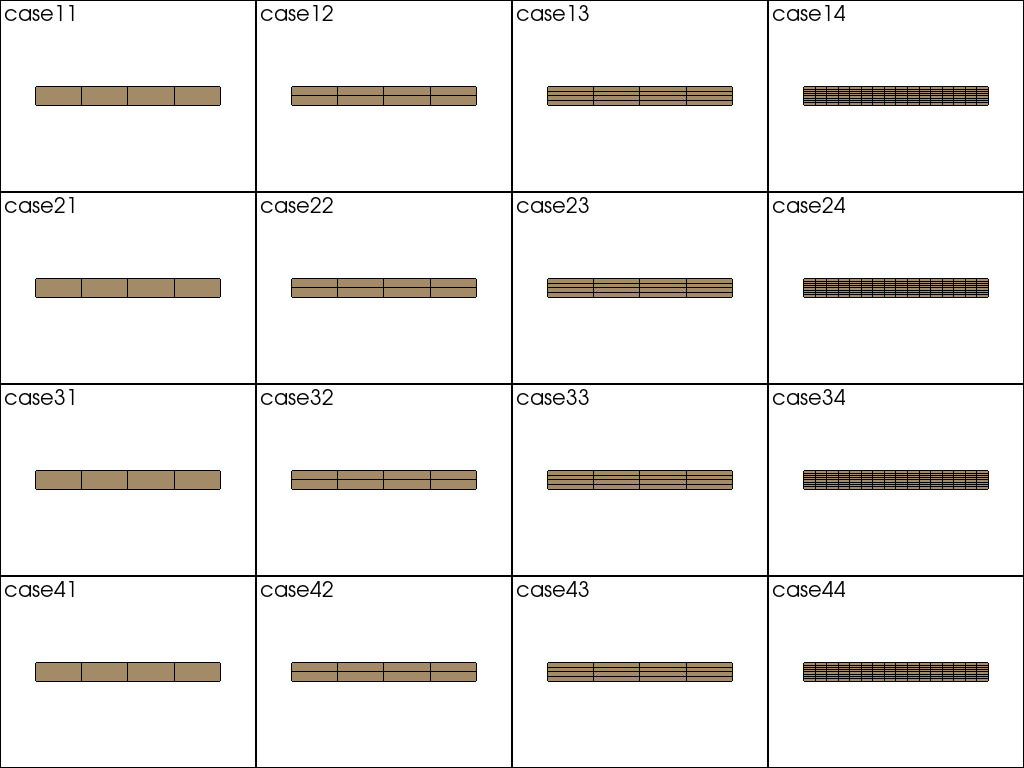
Outputs an image of each mesh.
[8]:
p = pv.Plotter(shape=(4, 4))

for i in range(4):
    for j in range(4):
        p.subplot(i, j)
        mesh = pv.read("mesh_" + cases[i * 4 + j] + ".vtk")
        p.add_text(cases[i * 4 + j], font_size=10)
        p.add_mesh(mesh, color="tan", show_edges=True)

p.show(cpos="xy")
[8]:
[(5.0, 0.5, 19.41486882686712),
 (5.0, 0.5, 0.0),
 (0.0, 1.0, 0.0)]
領域
Sets the area on the left side of the mesh where the Dirichlet condition is set. The right side sets the area for setting the Neumann condition.
[9]:
TOP_BOUND = 1
RIGHT_BOUND = 2
LEFT_BOUND = 3
BOTTOM_BOUND = 4

for mesh in meshs:
    fb1 = mesh.outer_faces_with_direction([0.0, 1.0], 0.01)
    fb2 = mesh.outer_faces_with_direction([1.0, 0.0], 0.01)
    fb3 = mesh.outer_faces_with_direction([-1.0, 0.0], 0.01)
    fb4 = mesh.outer_faces_with_direction([0.0, -1.0], 0.01)
    mesh.set_region(TOP_BOUND, fb1)
    mesh.set_region(RIGHT_BOUND, fb2)
    mesh.set_region(LEFT_BOUND, fb3)
    mesh.set_region(BOTTOM_BOUND, fb4)
有限要素法
Create a MeshFem object and associate the mesh with the finite element method.
[10]:
fems = []
for fem_name in fem_names:
    fems.append(gf.Fem("FEM_PRODUCT(" + fem_name + "," + fem_name + ")"))
[11]:
mfus = []
for mesh, fem in zip(meshs, fems):
    mfu = gf.MeshFem(mesh, 2)
    mfu.set_fem(fem)
    mfus.append(mfu)
Integral method
Associate the integration method with the mesh.
[12]:
ims = []
for method in methods:
    ims.append(gf.Integ("IM_PRODUCT(" + method + ", " + method + ")"))
[13]:
mims = []
for mesh, im in zip(meshs, ims):
    mim = gf.MeshIm(mesh, im)
    mims.append(mim)
Variable
Define the model object and set the variable 「u」.
[14]:
mds = []
for mfu in mfus:
    md = gf.Model("real")
    md.add_fem_variable("u", mfu)
    mds.append(md)
Properties
Define properties as constants for the model object. The Young’s modulus of steel is \(E = 205000\times 10^6N/m^2\). Also set Poisson’s ratio \(\nu = 0.0\) to ignore the Poisson effect.
[15]:
E = 10000  # N/mm2
Nu = 0.0

for md in mds:
    md.add_initialized_data("E", E)
    md.add_initialized_data("Nu", Nu)
Plane Strain Element
Defines the plane strain element for variable 『u』.
[16]:
for md, mim in zip(mds, mims):
    md.add_isotropic_linearized_elasticity_brick_pstrain(mim, "u", "E", "Nu")
Boundary Conditions
Set the Dirichlet condition for the region on the left side.
[17]:
for (md, mim, mfu, fem) in zip(mds, mims, mfus, fems):
    if fem.is_lagrange():
        md.add_Dirichlet_condition_with_simplification("u", LEFT_BOUND)
    else:
        md.add_Dirichlet_condition_with_multipliers(mim, "u", mfu, LEFT_BOUND)
Set the Neumann boundary condition on the right side.
[18]:
F = 1.0  # N/mm2
for (md, mfu, mim) in zip(mds, mfus, mims):
    md.add_initialized_data("F", [0, F / (b * h)])
    md.add_source_term_brick(mim, "u", "F", RIGHT_BOUND)
Solve
Solve the simultaneous equations of the model object to find the value of the variable 『u』.
[19]:
for md in mds:
    md.solve()
The constraint on the left end has a displacement of 0.0.
[20]:
for md, mfu, case in zip(mds, mfus, cases):
    u = md.variable("u")
    dof = mfu.basic_dof_on_region(LEFT_BOUND)
    npt.assert_almost_equal(abs(np.max(u[dof])), 0.0)
Review results
Output and visualize the results of each case to vtk files.
[21]:
for md, mfu, case in zip(mds, mfus, cases):
    u = md.variable("u")
    mfu.export_to_vtk("u_" + case + ".vtk", "ascii", mfu, u, "u")
Computation of Theoretical Solutions
Calculates the deflection at each coordinate for comparison with the theoretical solution. The theoretical solution for a cantilever beam subjected to a concentrated load is as follows.
\(w\left(x\right)=\dfrac{FL^3}{3EI}\)
[22]:
I = b * h ** 3 / 12
w = F * L ** 3 / (3 * E * I)
w
[22]:
0.4
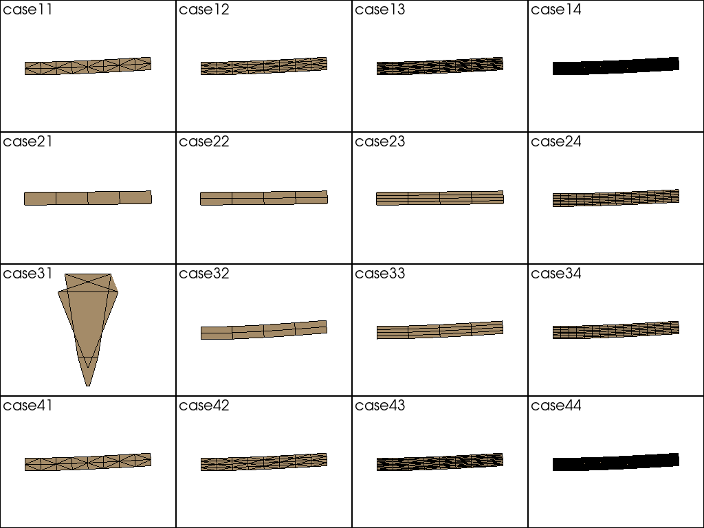
deformation diagram of case11
[23]:
p = pv.Plotter(shape=(4, 4))

for i in range(4):
    for j in range(4):
        p.subplot(i, j)
        mesh = pv.read("u_" + cases[i * 4 + j] + ".vtk")
        p.add_text(cases[i * 4 + j], font_size=10)
        p.add_mesh(mesh.warp_by_vector("u"), color="tan", show_edges=True)

p.show(cpos="xy")
[23]:
[(5.015016078948975, 0.7012025117874146, 19.565021099812608),
 (5.015016078948975, 0.7012025117874146, 0.0),
 (0.0, 1.0, 0.0)]
Comparison with Theoretical Solutions
[24]:
b = 1.0
I = b * h ** 3.0 / 12.0
dmax = 1.0 / 3.0 * (F * L ** 3) / (E * I)
dmax
[24]:
0.4
Calculates the ratio of deformation to theoretical solution for each case.
[25]:
data = []

columns = [
    "case name",
    "mesh",
    "finite element method",
    "integration method",
    "ratio with theory",
]

for case, x, y, fem_name, method, md, mfu in zip(
    cases, xs, ys, fem_names, methods, mds, mfus
):
    u = md.variable("u")
    dof = mfu.basic_dof_on_region(RIGHT_BOUND)
    ratio = "{:.3f}".format(max(u[dof] / dmax))
    data.append([case, str(x) + "x" + str(y), fem_name, method, ratio])
df = pd.DataFrame(data=data, columns=columns)
Markdown(df.to_markdown())
[25]:
| case name | メッシュ | 有限要素法 | 積分法 | ratio with theory | |
|---|---|---|---|---|---|
| 0 | case11 | 4x1 | FEM_PK(1, 2) | IM_GAUSS1D(4) | 0.999 |
| 1 | case12 | 4x2 | FEM_PK(1, 2) | IM_GAUSS1D(4) | 1 |
| 2 | case13 | 4x4 | FEM_PK(1, 2) | IM_GAUSS1D(4) | 1 |
| 3 | case14 | 16x8 | FEM_PK(1, 2) | IM_GAUSS1D(4) | 1.006 |
| 4 | case21 | 4x1 | FEM_PK(1, 1) | IM_GAUSS1D(2) | 0.244 |
| 5 | case22 | 4x2 | FEM_PK(1, 1) | IM_GAUSS1D(2) | 0.244 |
| 6 | case23 | 4x4 | FEM_PK(1, 1) | IM_GAUSS1D(2) | 0.244 |
| 7 | case24 | 16x8 | FEM_PK(1, 1) | IM_GAUSS1D(2) | 0.841 |
| 8 | case31 | 4x1 | FEM_PK(1, 1) | IM_GAUSS1D(0) | 6.52355e+10 |
| 9 | case32 | 4x2 | FEM_PK(1, 1) | IM_GAUSS1D(0) | 1.317 |
| 10 | case33 | 4x4 | FEM_PK(1, 1) | IM_GAUSS1D(0) | 1.056 |
| 11 | case34 | 16x8 | FEM_PK(1, 1) | IM_GAUSS1D(0) | 1.021 |
| 12 | case41 | 4x1 | FEM_PK_WITH_CUBIC_BUBBLE(1, 1) | IM_GAUSS1D(4) | 0.999 |
| 13 | case42 | 4x2 | FEM_PK_WITH_CUBIC_BUBBLE(1, 1) | IM_GAUSS1D(4) | 1 |
| 14 | case43 | 4x4 | FEM_PK_WITH_CUBIC_BUBBLE(1, 1) | IM_GAUSS1D(4) | 1 |
| 15 | case44 | 16x8 | FEM_PK_WITH_CUBIC_BUBBLE(1, 1) | IM_GAUSS1D(4) | 1.006 |
[ ]: