Introduction to FEM Analysis with Python

This tutorial aims to show using Python to pre-processing, solve, and post-processing of Finite Element Method analysis. It uses a finite element method library with a Python interface called GetFEM for preprocessing and solving. We will load vtk file by using meshio and visualize by matplotlib in pre-processing and post-processing. This tutorial was used in the PyConJP 2019 talk. You can watch the talk on YouTube below. This tutorial is based on the following official GetFEM page tutorial.

from IPython.display import YouTubeVideo

YouTubeVideo("6JuB1GiDLQQ", start=512)

Installation

GetFEM including its python interface can be installed from a terminal by executing aptitude update and aptitude install python3-getfem++.

sudo aptitude install python3-getfem++

The additional packages in requirements.txt are required for this tutorial. You do not need to build these environments because they are already configured in the Dockerfile.

The problem setting

The problem refers to “Poisson’s Equation on Unit Disk” published by Math Works’s homepage.

\[−\Delta u=1 \ {\rm on}\ \Omega, u=0 \ {\rm on}\ \delta \Omega\]

|pdedemo1\_01|

How to use GetEM

We take the following steps when using GetFEM to solve finite element problems. See this page for more information on using GetFEM.

• define a MesherObject
• define a Mesh
• define a MeshFem
• define a MeshIm
• define a Model and set it up
• solve Model object
• get value from Model object

Initialization

GetFEM can be imported as follows (numpy has also to be imported).

import getfem as gf
import numpy as np

Mesh generation

We use GetFEM’s MesherObject to create a mesh from the geometric information to be analyzed. This object represent a geometric object to be meshed by the experimental meshing procedure of GetFEM. We can represent a disk by specifying a radius, a 2D center, and using “ball” geometry.

center = [0.0, 0.0]
radius = 1.0

mo = gf.MesherObject("ball", center, radius)

We can make mesh object mesh by calling the experimental mesher of GetFEM on the geometry represented by mo. The approximate element diameter is given by h and the degree of the mesh is K (\(K > 1\) for curved boundaries).

h = 0.1
K = 2
mesh = gf.Mesh("generate", mo, h, K)

Boundary selection

To define a boundary condition, we set a boundary number on the outer circumference of the circle.

outer_faces = mesh.outer_faces()
OUTER_BOUND = 1
mesh.set_region(OUTER_BOUND, outer_faces)

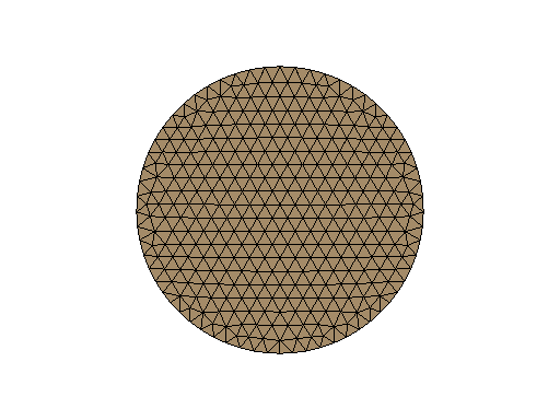
Mesh draw

We visualize the created mesh to check its quality. We can output mesh objects, but matplotlib can only display triangles. Therefore, we make a Slice object with a slice operation of ("none",), which does not cut the mesh. With a refinement of 1, this serves to convert the mesh to triangles.

sl = gf.Slice(("none",), mesh, 1)

We can export a slice to VTK file by using export_to_vtk method.

sl.export_to_vtk("sl.vtk", "ascii")

We can render VTK files using Paraview or mayavi2. In order to display in the jupyter notebook this time, we read in meshio and draw in matplotlib.

import pyvista as pv
from pyvirtualdisplay import Display

display = Display(visible=0, size=(1280, 1024))
display.start()
p = pv.Plotter()
m = pv.read("sl.vtk")
p.add_mesh(m, show_edges=True)
pts = m.points
p.show(window_size=[512, 384], cpos="xy")
display.stop()

<pyvirtualdisplay.display.Display at 0x7f96ba6ef160>

Definition of finite element methods and integration method

We define the finite element and integration methods to use. We create a MeshFem that defines the degree of freedom of the mesh as rank 1 (scalar).

mfu = gf.MeshFem(mesh, 1)

Next we set the finite element used. Classical finite element means a continuous Lagrange element. Setting elements_degree to 2 means that we will use quadratic (isoparametric) elements.

elements_degree = 2
mfu.set_classical_fem(elements_degree)

The last thing to define is an integration method mim. There is no default integration method in GetFEM so it is mandatory to define an integration method. Of course, the order of the integration method has to be chosen sufficient to make a convenient integration of the selected finite element method. Here, the square of elements_degree is sufficient.

mim = gf.MeshIm(mesh, pow(elements_degree, 2))

Model definition

The model object in GetFEM gathers the variables of the models (the unknowns), the data and what are called the model bricks. The model bricks are some parts of the model (linear or nonlinear terms) applied on a single variable or linking several variables. A model brick is an object that is supposed to represent a part of a model. It aims to represent some integral terms in a weak formulation of a PDE model. They are used to make the assembly of the (tangent) linear system (see The model object for more details).

\[[K] \left\{ u \right\} = \left\{ F \right\}\]

md = gf.Model("real")
md.add_fem_variable("u", mfu)

Poisson’s equation

To define Poisson’s equation, we have to define a Laplacian term and RHS source term. We can add the Laplacian term (which is called a brick in GetFEM) by using add_Laplacian_brick().

md.add_Laplacian_brick(mim, "u")

0

If you want to define constants in GetFEM, we use the add_fem_data() method.

F = 1.0
md.add_fem_data("F", mfu)

We can set constant values with the set_variable() method. Here we pass a vector (ndarray) the size of the degrees of freedom.

md.set_variable("F", np.repeat(F, mfu.nbdof()))

We define the term RHS with the add_source_term_brick() method, using the constant F just defined.

md.add_source_term_brick(mim, "u", "F")

1

Finally, we set the Dirichlet condition at the boundary.

md.add_Dirichlet_condition_with_multipliers(mim, "u", elements_degree - 1, OUTER_BOUND)

2

Model solve

Once the model is correctly defined, we can simply solve it by:

md.solve()

(0, 1)

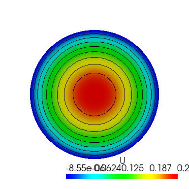
Export/visualization of the solution

The finite element problem is now solved. We can get the solution \(u\) by using variable method.

U = md.variable("u")

We can output the computed u with the mesh of the Slice object.

sl.export_to_vtk("u.vtk", "ascii", mfu, U, "U")

display = Display(visible=0, size=(1280, 1024))
display.start()
p = pv.Plotter()
m = pv.read("u.vtk")
contours = m.contour()
p.add_mesh(m, show_edges=False)
p.add_mesh(contours, color="black", line_width=1)
p.add_mesh(m.contour(8).extract_largest(), opacity=0.1)
pts = m.points
p.show(window_size=[384, 384], cpos="xy")
display.stop()

<pyvirtualdisplay.display.Display at 0x7f968c03a760>

Exact solution

The exact solution to this problem is given by the following equation:

\[u(x, y) = \dfrac{1-x^2-y^2}{4}\]

evalue = mfu.eval("(1-x*x-y*y)/4")

We can calculate the error for the L2 and H1 norms by using compute:

L2error = gf.compute(mfu, U - evalue, "L2 norm", mim)
H1error = gf.compute(mfu, U - evalue, "H1 norm", mim)
print("Error in L2 norm : ", L2error)
print("Error in H1 norm : ", H1error)

Error in L2 norm :  1.965329030567132e-06
Error in H1 norm :  0.00010936971229957788

As you can see, the size of the error is within the acceptable range.

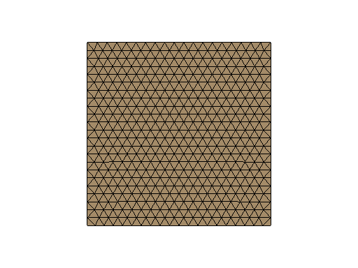
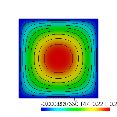
Quadrangular shape case

Even if the shape of the region is different, GetFEM can obtain a finite element solution by rewriting the program a little. In the case of a quadrangular shape it may be calculated for:.

# Mesh generation
mo = gf.MesherObject("rectangle", [-1.0, -1.0], [1.0, 1.0])
h = 0.1
K = 2
mesh = gf.Mesh("generate", mo, h, K)

# Boundary selection
outer_faces = mesh.outer_faces()
OUTER_BOUND = 1
mesh.set_region(OUTER_BOUND, outer_faces)
sl = gf.Slice(("none",), mesh, 1)
sl.export_to_vtk("sl.vtk", "ascii")

# Mesh draw
display = Display(visible=0, size=(1280, 1024))
display.start()
p = pv.Plotter()
m = pv.read("sl.vtk")
p.add_mesh(m, show_edges=True)
pts = m.points
p.show(window_size=[512, 384], cpos="xy")
display.stop()

<pyvirtualdisplay.display.Display at 0x7f96ba6dd040>

# Definition of finite element methods and integration method
mfu = gf.MeshFem(mesh, 1)
elements_degree = 2
mfu.set_classical_fem(elements_degree)
mim = gf.MeshIm(mesh, pow(elements_degree, 2))

# Model definition
md = gf.Model("real")
md.add_fem_variable("u", mfu)

# Poisson’s equation
md.add_Laplacian_brick(mim, "u")
F = 1.0
md.add_fem_data("F", mfu)
md.set_variable("F", np.repeat(F, mfu.nbdof()))
md.add_source_term_brick(mim, "u", "F")
md.add_Dirichlet_condition_with_multipliers(mim, "u", elements_degree - 1, OUTER_BOUND)

# Model solve
md.solve()

# Export/visualization of the solution
U = md.variable("u")
sl.export_to_vtk("u.vtk", "ascii", mfu, U, "U")

display = Display(visible=0, size=(1280, 1024))
display.start()
p = pv.Plotter()
m = pv.read("u.vtk")
contours = m.contour()
p.add_mesh(m, show_edges=False)
p.add_mesh(contours, color="black", line_width=1)
p.add_mesh(m.contour(8).extract_largest(), opacity=0.1)
pts = m.points
p.show(window_size=[384, 384], cpos="xy")
display.stop()

<pyvirtualdisplay.display.Display at 0x7f9694d31730>